Machine Learning @ Coursera
A cheat sheet
This cheatsheet wants to provide an overview of the concepts and the used formulas and definitions of the »Machine Learning« online course at coursera.
Last changed:
Please note: I changed the notation very slighty. I'll denote vectors with a little arrow on the top. Example: $\vec\theta$
The octave tutorial that was part of the seond week is available as a script here.
Week 1
Introduction
Machine Learning
»Well-posed Learning Problem: A computer program is said to learn from experience E with respect to some task T and some performance measure E, if its performance on T, as measured by P, improves with experience E.«
— Tom Mitchell (1998) [1]
Supervised Learning
Supervised learning is the task of learning to predict the answers for unseen examples where the right answers for some examples are given to learn from.
Unsupervised Learning
Unsupervised learning is learning in the absence of right answers to learn from. The algorithm discovers structure in the data on its own.
Regression Problem
Regression problems need estimators to predict continuous output, such as house prices.
Classification Problem
Classification problems need estimators to predict categorical (discrete) valued output. (I.e. $0$ or $1$, whether or not a patient has cancer or not.)
Linear Regression with One Variable
Model Representation
Notations:
- $m$: number of training examples
- $x$'s: input variable/features
- $y$'s: output variables/target
- $(x,y)$: one training example
- $(x^{(i)},y^{(i)})$: $i$th training example
Univariate Hypothesis
The hypothesis function maps x's to y's ($h: x \mapsto y$). It can be represented by:
$$h_{\theta} = \theta_{0} + \theta_{1}x$$The shorthand for the hypothesis is $h(x)$. $\theta_{i}$'s are called the parameters of the hypothesis. In this case the hypothesis is called »Univariate Linear Regression«.
Cost Function
Idea: Choose $\theta_0, \theta_1$ so that $h_\theta(x)$ is close to $y$ for our training examples $(x,y)$. The 3D-surface plot below visualizes the cost function for the two parameters.
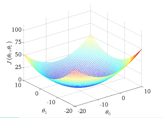
Squared Error Cost Function
$$J(\theta_0, \theta_1) = \frac{1}{2m} \sum^{m}_{i=1}\left(h_{\theta}(x^{(i)}) - y^{(i)}\right)^2$$The Gradient Descent Algorithm
The goal is to choose the hypothises' parameters in a manner that the the output of the cost function $J(\theta_0, \theta_1)$ is minimal.
Outline:
- Start with some $\theta_0, \theta_1$
- Keep changing $\theta_0, \theta_1$ to reduce $J(\theta_0, \theta_1)$ until we hopefully end up at a minimum
Gradient Descent Algorithm
Note that the values of $\theta_0$ and $\theta_1$ are updated simultaneously. $\alpha$ is called the learning rate.
$$\begin{aligned} \text{repeat} & \text{ until convergence} \; \{\\ & \theta_j := \theta_j - \alpha \frac{\delta}{\delta\theta_j} J(\theta_0, \theta_1) \;\; \text{(for j=0 and j=1)}\\ \} \phantom{15pt} & \end{aligned}$$The correct implementation of the simultaneous update looks like this:
$$\begin{aligned} & temp0 := \theta_0 - \alpha \frac{\delta}{\delta\theta_j} J(\theta_0, \theta_1)\\ & temp1 := \theta_1 - \alpha \frac{\delta}{\delta\theta_j} J(\theta_0, \theta_1)\\ & \theta_0 := temp0 \\ & \theta_1 := temp1 \end{aligned}$$Partial derivitive of the cost function
$$\begin{aligned} \text{repeat} & \text{ until convergence} \; \{\\ & \theta_0 := \theta_0 - \alpha \frac{1}{m} \sum^{m}_{i=0}\left(h_\theta(x^{(i)}) - y^{(i)}\right)\\ & \theta_1 := \theta_1 - \alpha \frac{1}{m} \sum^{m}_{i=0}\left(h_\theta(x^{(i)}) - y^{(i)}\right) \cdot x^{(i)}\\ \} \phantom{15pt} & \end{aligned}$$Note: The cost function $J(\theta_0, \theta_1)$ is convex and therefore has only one optimum overall.
Batch Gradient Descent
If the gradient descent uses all $m$ training examples in each iteration it is also called Batch Gradient Descent Algorithm.
Week 2
Linear Regression with Multiple Variables
Multiple Features
Notations:
- $n$: number of features
- $\vec x^{(i)}$: input features of ith training example
- $x^{(i)}_j$: value of feature $j$ in ith training example
Multivariate Hypothesis
$$h_\theta = \theta_0 + \theta_1 x_1 + \theta_2 x_2 + \cdots + \theta_n x_n$$For convenience of notation we'll define $x_0 = 1$ ($x_0^{(i)}$). Thus a feature vector looks like:
$$ \vec x = \left[\begin{array}{c} x_0\\ x_1 \\ \vdots \\ x_n \end{array}\right] \in \mathbb{R}^{n+1}$$And the parameters can be written as:
$$ \vec \theta = \left[\begin{array}{c} \theta_0\\ \theta_1 \\ \vdots \\ \theta_n \end{array}\right] \in \mathbb{R}^{n+1}$$The hypothesis can now be written as:
$$\begin{align} h_\theta & = \theta_0 x_0 + \theta_1 x_1 + \theta_2 x_2 + \cdots + \theta_n x_n\\ & = \left[ \theta_0 \theta_1 \cdots \theta_n \right] \left[\begin{array}{c} \theta_0\\ \theta_1 \\ \vdots \\ \theta_n \end{array}\right] \\ & = \boxed{\vec\theta^{T}\vec x}\\ \end{align}$$This hypothesis is called »Multivariate Linear Regression«.
Gradient Descent for Multiple Variables
The cost function can now be written as:
$$\begin{aligned} J(\theta_0, \theta_1, ..., \theta_n) & = \frac{1}{2m}\sum^{m}_{i=1} \left(h_\theta(x^{(i)}) - y^{(i)}\right)^2\\ & = \boxed{J(\vec\theta)} \end{aligned}$$The gradient descent algorithm for this cost function looks like this:
$$\begin{aligned} \text{repeat} & \{\\ & \theta_j := \theta_j - \alpha \frac{\delta}{\delta \theta_j} \; \; J(\theta_0, \theta_1, ... , \theta_n)\\ \} \phantom{15pt} & \end{aligned}$$Which can also be written like this:
$$\begin{aligned} \text{repeat} & \{\\ & \theta_j := \theta_j - \alpha \frac{1}{m} \sum^{m}_{i=1}\left( h_\theta(\vec x^{(i)}) -y^{(i)} \right) x_j^{(i)}) \\ \} \phantom{15pt} & \end{aligned}$$Again, the parameters $\theta_j \; \forall j= 0, ..., n$ have to be updated simultaneously.
Feature Scaling
Get every feature into approximately a $-1 \leq x_i \leq 1$ range to optimize the path finding of the gradient descent algorithm.
Mean Normalization
Replace $x_i$ with $x_i - \mu_i$ to make features have approximately zero mean (does not apply to $x_0 = 1$).
$$x_1 \leftarrow \frac{x_1 - \mu_1}{s_1}$$where $\mu_1$ is the average value of x in the training set and $s_1$ is the range $max - min$ (or standard deviation).
Learning Rate $\alpha$
General rule: $J(\vec\theta)$ should decrease after every iteration.
Example Automatic Convergence Test
Declare convergence if $J(\vec\theta)$ decreases by less than $\epsilon = 10^{-3}$ in one iteration.
Make sure gradient descent works correctly:
- If $\alpha$ is too small: slow convergence
- If $\alpha$ is too large: $J(\vec\theta)$ may not decrease on every iteration and may not converge
For $\alpha$ try: $0.001$, $0.003$, $0.01$, $0.03$, $0.1$, $0.3$, $1$ etc.
Features and Polynomial Regression
You can choose your model to fit to a polynomial if you want it to behave in a specific way. You not only can choose to multiply/divide two or more features to create a new feature, you can also fit your model to a more complex polynomial. If you want your model to behave for example to increase you could choose to use $(size)^2$, fit it to a cubic polynomial the same way, or use $\sqrt{size}$.
Normal Equation
An alternative to the gradient descent algorithm is an analytical solution to minimize the cost function $J(\vec\theta)$.
$$\theta \in \mathbb{R}^{n+1} \;\;\; J(\theta_0, \theta_1, \cdots, \theta_m) = \frac{1}{2m}\sum^{m}_{i=1} \left( h_\theta(x^{(i)} - y^{(i)}\right)^2$$ $$\frac{\delta}{\delta\theta_j} J(\vec\theta) = \cdots = 0 \;\;\; \text{(for every $j$)}$$Then solve for $\theta_0,\theta_1,\cdots,\theta_n$ by setting the equation to equal zero. For $m$ examples $(\vec x^{(i)}, y^{(i)}), \cdots, (\vec x^{(m)}, y^{(m)})$ with $n$ features the input feature of the ith training example looks like this:
$$\vec x^{(i)} = \left[ \begin{array}{c} x_0^{(i)}\\ x_1^{(i)} \\ \vdots \\ x_n^{(i)} \end{array} \right] \in \mathbb{R}^{n+1}$$The design matrix $x$ then looks like that:
$$ X = \left[ \begin{array}{c} (x^{(1)})^T \\ (x^{(2)})^T \\ \vdots \\ (x^{(m)})^T \end{array} \right]$$and the vector of the outputs of the training examples look like this:
$$ \vec y = \left[ \begin{array}{c} y^{(1)} \\ y^{(2)} \\ \vdots \\ y^{(m)}\end{array}\right]$$With the design matrix the minimum $\vec \theta$ is:
$$ \vec \theta = (X^TX)^{-1} X^T \vec y$$Note: using this method you don't need to scale the features.
Gradient Descent versus Normal Equation
For $m$ training examples and $n$ features:
Gradient Descent:
- Need to choose $\alpha$
- Needs many iterations
- Works well even when $n$ is large
Normal Equation
- No need to choose $\alpha$
- Don't need to iterate
- Need to compute $(X^TX)^{-1})$ (complexity $O(n^3)$)
- Slow if $n$ is very large
Normal Equation Noninvertibility
Although very rarely, it can happen that $X^TX$ is non-invertible, for example if the matrix is singular or degenerate.
Problems can be that redundant features are used (and therefore the vetors are linearly dependent) or that too many features are used (e.g. $m \leq n$). The solution for that would be to delete some features or use regularization (which comes later in this course).
Week 3
Linear Regression
With $y \in \{0, 1\}$ the linear regression model is
$$0 \leq h_\theta(x) \leq 1$$Hypothesis for Logistic Regression Models
The hypothesis for this model is this:
$$h_\theta(x) = g(\theta^Tx)$$Where $g$ is called sigmoid function or logistic function
$$g(z) = \frac{1}{1+e^{-z}}$$Which gives us the following representation for the hypothesis:
$$h_\theta(x) = \frac{1}{1+e^{-\theta^Tx}}$$Interpretation of the Hypothesis Output
$h_\theta(x)$ is the estimated probability that $y=1$ on input $x$:
$$h_\theta(x) = P(y = 1 | x ; \theta)$$Which reads like probability that $y=1$ given x, parameterized by $\theta$
$$P(y=0|x;\theta) + P(y=1|x;\theta) = 1\\ P(y=0|x;\theta) = 1 - P(y=1|x;\theta)$$Decision Boundary
Suppose we predict $y=1$ if $h_\theta(x) \geq 0.5$. $g(z) \geq 0.5 $ when $z \geq 0$. For $h_\theta(x) = g(\theta^Tx) \geq 0.5$ whenever $z = \theta^Tx \geq 0$. Suppose we predict $y=0$ if $h_\theta(x) < 0.5$.
The decision boundary ist part of the hypothesis. If we for example have a hypothesis with two features, the term $\theta_0 + \theta_1 x_1 + \theta_2 x_2$ gives the decision boundary, where this is the hypothesis:
$$h_\theta(x) = g(\theta_0 + \theta_1 x_1 + \theta_2 x_2)$$Non-linear Decision Boundaries
As previously mentioned one can add custom features to fit the hypothesis to the data. This allows us to add custom features that result in a circular decision boundary.
For example:
$$\vec \theta = \left[\begin{array}{c} -1\\ 0 \\ 0 \\ 1 \\ 1 \end{array}\right]\\$$With custom features $x_1^2$ and $x_2^2$:
$$h_\theta(x) = \theta_0 + \theta_1 x_1 + \theta_2 x_2 + \theta_3 x_1^2 + \theta_4 x_2^2$$We predict $y=1$ if $-1 + x^2_1 + x^2_2 \geq 0$. The polynom can have as much custom features as you wish to fit the data. Even with non-circular non-linear decision boundaries.
Cost Function
Notation:
- Training set: $\left\{ (x^{(1)}, y^{(1)}), (x^{(2)}, y^{(2)}), \cdots, (x^{(m)}, y^{(m)})\right\}$
- $m$ examples $\;\;\;x \in \left[\begin{array}{c} x_0\\ x_1 \\ \vdots \\ x_n \end{array}\right] \; \; \; x_0 = 1, y \in \{0,1\}$
- $h_\theta = \frac{1}{1+e^{-\theta^Tx}}$
The cost function for linear regression was:
$$J(\vec\theta) = \frac{1}{m} \sum^m_{i=1} \frac{1}{2}\left(h_\theta(x^{(i)}) - y^{(i)}\right)^2 = cost(h_\theta(x^{(i)}), y^{(i)})\\ cost(h_\theta(\vec x), \vec y) = \frac{1}{2}(h_\theta(\vec x) - \vec y)^2$$This cost function is non-convex. For logistic regression we want a convex function.
$$cost(h_\theta(\vec x), \vec y) = \left\{ \begin{array}{r} -log(h_\theta(\vec x)) \;\;\; \text{if} \;\; y = 1 \\ -log(1 - h_\theta(\vec x)) \;\;\; \text{if} \;\; y = 0\end{array}\right.$$If the $\text{cost} \, = 0 \; \text{if} \; y = 1, h_\theta(x) = 1$ but as $h_\theta(x) \rightarrow 0$ $Cost \rightarrow \infty$. This captures the intuition that if $h_\theta(x) = 0$ (predict $P(y=1|x;\theta)$), but $y=1$ we'll penalize the learning alrogithm by a very large cost.
Simplified Cost Function and Gradient Descent
The cost function can be simplified to a one liner:
$$cost(h_\theta(x),x) = -y \; log(h_\theta(x)) - (1-y) log(1-h_\theta(x))$$This works because if $y=1$, the first term will be multiplicated by $1$ and the second term will be multiplicated with $(1-y) = (1-1) = 0$. If $y=0$ the first term is multiplicated with 0 and the second term is multiplicated with $(1-0) = 1$.
This gives us the complete cost function $J(\vec\theta)$:
$$\begin{align} J(\vec\theta) & = \frac{1}{m} \sum^m_{i=1} cost(h_\theta(x^{(i)}),y^{(i)})\\ & = - \frac{1}{m} \left[\sum^m_{i=1} y^{(i)} log(h_\theta(x^{(i)})) + (1-y^{(i)} ) log(1 - h_\theta( x^{(i)}))\right] \end{align}$$To fit parameters $\vec\theta$ $\text{min}_\theta J(\vec\theta)$ is calculated. To make a new prediction given new x the output of $h_\theta$ has to be calculated ($P(y=1|x;\theta)$).
Gradient Descent
$\text{min}_\theta J(\theta)$:
$$\begin{aligned} \text{repeat} &\{\\ & \theta_j := \theta_j - \alpha \sum^m_{i=1} (h_\theta(x^{(i)}) - y^{(i)})x_j^{(i)}\\ \} \phantom{15pt} & \end{aligned}$$Advanced Optimization
In general we need to compute two things for our optimization:
- $J(\vec \theta)$
- $\frac{\delta}{\delta\theta_j}J(\vec \theta)$
Besides gradient descent, there are several other algorithms that could be used:
- Conjugate Gradient
- BFGS
- L-BFGS
The advantages:
- No need to manually pick $\alpha$
- Often faster than gradient descent
The disadvantages:
- More complex
Example for $\text{min}_\theta$
$$\vec\theta=\left[\begin{array}{c} \theta_1 \\ \theta_2 \end{array}\right]\\ J(\vec\theta) = (\theta_1 -5)^2 + (\theta_2 -5)^2\\ \frac{\delta}{\delta\theta_1}=2(\theta_1 -5)\\ \frac{\delta}{\delta\theta_2} = 2(\theta_2 - 5)$$function[jVal, gradient] = costFunction(theta)
% code to compute J(theta)
jVal = (theta(1) - 5)^2 + (theta(2)-5)^2;
gradient = zeros(2,1);
% code to compute delta/delta theta_j J(theta)
gradient(1) = 2*(theta(1)-5);
gradient(2) = 2*theta(2)-5);
options = optimset('GradObj', 'on', 'MaxIter', '100');
initialTheta = zeros(2,1);
[optTheta, functionval, exitFlag] = fminunc(@costFunction, initialTheta, options);Multiclass Classification: One-vs-all
Classification with more than two $y$'s works like this:
$$h_\theta^{(i)}(x) = P(y=i|x;\theta) \;\;\; (i = 1,2,3,...)$$Each $i$ has it's own hypothesis $h_\theta^{(i)}(x)$ and predicts the probability that $y=i$ for each class $i$. On a new input $x$, to make a prediction, pick the class $i$ that maximizes $\text{max}_i h_\theta^{(i)}(x)$
Regularization
To prevent overfitting or underfitting of our hypothesis, we can regularize regressions.
Regularized Linear Regression
$$J(\vec\theta) = \frac{1}{2m} \left[\sum^m_{i=1}(h_\theta(x^{(i)}) -y^{(i)})^2 + \lambda \sum^m_{j=1}\theta_j \right]$$Where the term prepended by $y$ is called the regularization term. The goal is again to $\text{min}_\theta \; J(\vec\theta)$. The regularized gradient descent looks like this:
$$\begin{aligned} \text{repeat} & \{\\ & \theta_0 := \theta_0 - \alpha \frac{1}{m} \sum^m_{i=0} (h_\theta(x^{(i)}) - y^{(i)})x_0^{(i)}\\ & \theta_j := \theta_j - \alpha \left[ \frac{1}{m} \sum^m_{i=0} (h_\theta(x^{(i)}) - y^{(i)})x^{(i)}_j + \frac{\lambda}{m} \theta_j \right] \;\; \text{(for j=1...n)}\\ \} \phantom{15pt} & \end{aligned}$$Note that $\theta_0$ does not get penalized for over- or underfitting and therefore not regularized. The second term simply is $\frac{\delta}{\delta \theta_j} J(\vec\theta)$. For $j > 0$ the term can also be written as:
$$\theta_j = \theta_j(1-\alpha \frac{\lambda}{m}) - \alpha \frac{1}{m} \sum^m_{i=0}(h_\theta(x^{(i)}) - y^{(i)})x^{(i)}_j$$You can see that written this way, the term is pretty much the same as the original term.
Regularized Normal Equation
$$X = \left[\begin{array}{c} (x^{(1)})^T \\ \vdots \\ (x^{(m)})^T \end{array}\right] \in \mathbb{R}^{mx(n+1)} \;\; \text{with} \;\; y = \left[\begin{array}{c} y^{(1)} \\ \vdots \\ y^{(m)} \end{array}\right] \in \mathbb{R}^{m}$$The regularized normal equation now looks like this:
$$\vec\theta = (X^T X + \lambda \left[\begin{array}{ccccc} 0 & 0 & 0 & \cdots & 0 \\ 0 & 1 & 0 & \cdots & 0 \\ 0 & 0 & 1 & \cdots & 0 \\ \vdots & \vdots & \vdots & \ddots & \vdots \\ 0 & 0 & 0 & \cdots & 1 \\ \end{array}\right])^{-1}X^T y$$Where the matrix consisting of zeros and ones is sized $(n+1)x(n+1)$.
Non-Invertibility
Suppose $m \leq n$ where $m$ is the number of examples and $n$ is the number of features.
$$\theta = (X^TX)^{-1}X^T y$$When $m \leq n$ $X^TX$ is not invertible.
If $\lambda > 0$ the matrix is invertible because of the regularization.
Regularized Logistic Regression
$$J(\vec \theta) = - \left[ \frac{1}{m} \sum^{m}_{i=1} log(h_\theta(x^{(i)})) + (1-y^{(i)})log(1- h_\theta(x^{(i)})) \right] + \frac{\lambda}{2m} \sum^m_{i=1} \theta^2_j$$To prevent overfitting, $\theta_j$ will be penalized with $y>0$ for being too large.
Week 4
Neural Networks: Representation
Non-Linear Hypothesis
For more complex hypothesis that are non-linear to fit the hypothesis it might be required to add a number of quadratic or other features. With a higher number of features, this results in a really large hypothesis. This is where neural networks come in.
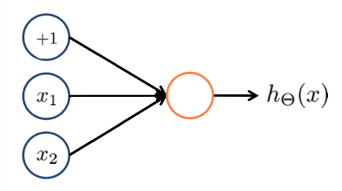
Model Representation I
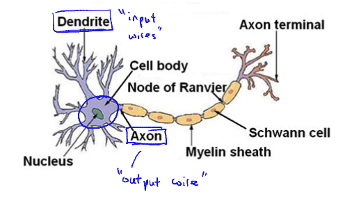
- Dendrite: input wires
- Axon: output wire
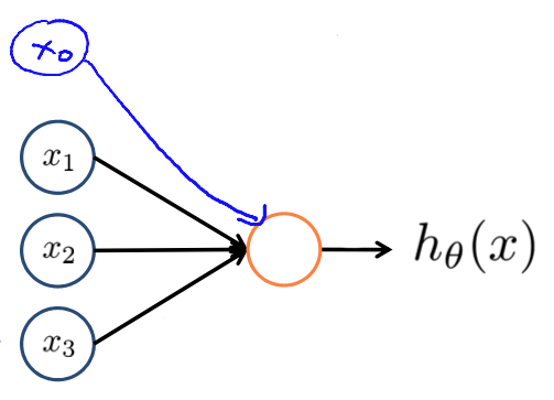
- Hypothesis: $h_\Theta(x) = \frac{1}{1+e^{-\Theta^Tx}}$ (also called sigmoid activation function)
- $x_0$: bias unit with $x_0 = 1$
The so called weights of the neurons are going to be the parameters of this model.
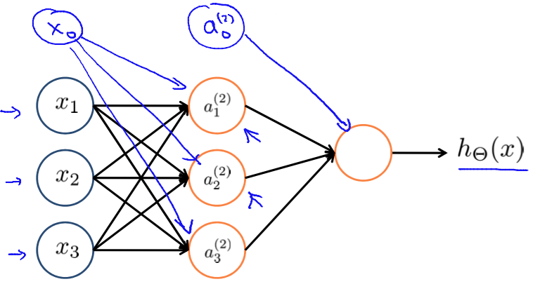
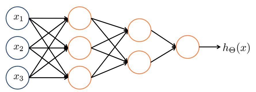
Again, $x_0$ and $a_0^(2)$ are the bias units. The first layer ($\{x_0, x_1, x_2, x_3\}$) is called the input layer. The third layer ($\{a^{(2)}_0, a^{(2)}_1, a^{(2)}_2, a^{(2)}_3\}$) is called the output layer. All layers between the input and the output layers are called hidden layers. So in this example, layer 2 is a hidden layer.
- $a^{(j)}_i$: activation of unit $i$ in layer $j$
- $\Theta^{(j)}$: matrix of weights controlling function mapping from layer $j$ to layer $j+1$
In general, if a network has $s_j$ units in layer $j$, $s_{j+1}$ units in layer $j+1$, then $\Theta^{(j)}$ will be of dimension $s_{j+1} \times (s_j+1)$
Model Representation II
Forward Propagation: Vectorized Implementation
From the first layer to the output layer the values are calculated based on the values of the previous layer.
$$x=\left[\begin{array}{c} x_0 \\ \vdots \\ x_3 \end{array}\right], \;\; z^{(2)}=\left[\begin{array}{c} z^{(2)}_1 \\ z^{(2)}_2 \\ z^{(2)}_3 \end{array}\right]$$With $z^{(2)} = \Theta^{(1)}a^{(1)}$ and $a^{(2)} = g(z^{(3)})$. Basically this is just a logistic regression for each layer $a_i^{(j)}$. For the bias unit we add $a^{(2)}_0 = 1$ ($\Rightarrow a^{(2)} \in \mathbb{R}^{n+1}$). $z^{(3)} = \Theta^{(2)}a^{(2)}$ and $h_\Theta(x) = a^{(3)} = g(z^{(3)})$.
Examples and Intuitition I
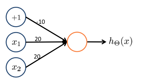
Simple Example: AND
- $x_1, x_2 \in \{0,1\}$
- $y = x_1 \text{AND} x_2$
We add the following weights to achieve the AND operation:
- $\Theta_{10}^{(1)} = -30$
- $\Theta_{11}^{(1)} = 20$
- $\Theta_{12}^{(1)} = 20$
$h_\Theta(x) = g(-30+20x_1+20x_2)$
| $x_1$ | $x_2$ | $h_\Theta(x)$ |
|---|---|---|
| $0$ | $0$ | $g(-30) \approx 0$ |
| $0$ | $1$ | $g(-10) \approx 0$ |
| $1$ | $0$ | $g(-10) \approx 0$ |
| $1$ | $1$ | $g(10) \approx 1$ |
Simple Example: OR
$h_\Theta(x) = g(-10 + 20x_1 + 20x_2)$
| $x_1$ | $x_2$ | $h_\Theta(x)$ |
|---|---|---|
| $0$ | $0$ | $g(-10) \approx 0$ |
| $0$ | $1$ | $g(10) \approx 1$ |
| $1$ | $0$ | $g(10) \approx 1$ |
| $1$ | $1$ | $g(30) \approx 1$ |
Examples and Intuitition II
Negation
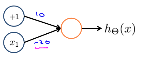
$h_\Theta(x) = g(10 - 20x_1)$
| $x_1$ | $h_\Theta(x)$ |
|---|---|
| $0$ | $g(10) \approx 1$ |
| $1$ | $g(-10) \approx 0$ |
XNOR

| $x_1$ | $x_2$ | $a_1^{(2)}$ | $a_2^{(2)}$ | $h_\Theta(x)$ |
|---|---|---|---|---|
| $0$ | $0$ | $0$ | $1$ | $1$ |
| $0$ | $1$ | $0$ | $0$ | $0$ |
| $1$ | $0$ | $0$ | $0$ | $0$ |
| $1$ | $1$ | $1$ | $1$ | $1$ |
Multiclass Classification
$y^{(i)}\in\mathbb{R}^n$ where $n$ is the number of classes.
$$h_\Theta = \left[\begin{array}{c} 0 \\ \vdots \\ 0 \\ 1 \\ 0 \\ \vdots 0 \end{array}\right]$$The $i$-th column is equal to $1$ for the $i$-th feature of the output layer.
Advanced Optimization
function[jVal ,gradient] = costFunction(gradient = [code to compute the partial derivitive of theta_j of J(theta)]; theta)With $j>1$ (note that octave indexes start at 1).
Neural Networks: Learning
Cost Function
$$\{ (x^{(1)}, y^{(1)}), …, (x^{(m)}, y^{(m)}) \}\\ L = \text{number of layers in network}\\ s_l = \text{numbers of units (that are not bias units)}$$Binary Classification
$y \in \{0,1\}$ with one output unit.
Multi-Class Classification
For $K$ classes: $y \in \mathbb{R}^K$ with $K$ output units.
Cost Function
The cost function for neural networks is similar to the regularized logistic regressions cost function.
$$ h_\Theta(x) \in \mathbb{R}^K \;\; (h_\Theta(x))_i = \text{i-th output}\\ $$ $$\begin{align} J(\Theta) = &-\frac{1}{m}\left[ \sum^{m}_{i=1} \sum^{K}_{k=1} y^{(i)}_k log(h_\Theta(x^{(i)}))_k + (1-y^{(i)}_k) log(1-(h_\Theta(x{(i)}))_k) \right]\\ & + \frac{\lambda}{2m} \sum^{L-1}_{l=1}\sum^{s_l}_{i=1}\sum^{s_{l+1}}_{j=1}(\Theta^{(l)}_{ji})^2 \end{align} $$Backpropagation Algorithm
Gradient Computation
With $J(\Theta)$ we now need $\text{min}_\Theta$. For that we need to compute:
- $J(\Theta)$
- $\frac{\delta}{\delta \Theta^{(l)}_{ij}} J(\Theta)$ with $\Theta^{(l)}_{ij} \in \mathbb{R}$
Intuitition: $\delta^{(l)}_j$ is the error of node $j$ in layer $l$. If we for example have a four layer network ($L = 4$) we have to calculate three errors:
- $\delta^{(4)}_j = a^{(4)}_j - y_j$ what basically is $\delta^{(4)} = h_\Theta(x) - y$
- $\delta^{(3)}_j = (\Theta^{(3)})^T \delta^{(4)} .* g'(z^{(3)})$
- $\delta^{(2)}_j = (\Theta^{(2)})^T \delta^{(3)} .* g'(z^{(2)})$
Alrogithm: Backpropagation
The training set is :$\{ (x^{(1)}, y^{(1)}), ..., (x^{(m)}, y^{(m)}) \}$. We now set $\Delta^{(l)}_{ij} = 0 \; \forall \; l,j,i$. $\Delta$ is used to compute $\frac{\delta}{\delta \Theta_{ij}^{(l)}} J(\Theta)$.
$$\begin{aligned} \text{for} \; & i = 1 \; \text{to} \; m\\ & \text{set} \; a^{(1)} = x^{(i)}\\ & \text{perform forward propagation to compute} \; a^{(l)} \; \text{for} \; l = 2,3,...,L\\ & \text{using} \; y^{(i)} \text{, compute} \delta^{(L)} = a^{(L)} - y^{(i)}\\ & \text{compute} \; \delta^{(L-1)}, \delta^{(L-2)}, ..., \delta^{(2)}\\ & \Delta^{(l)}_{ij} := \Delta^{(l)}_{ij} + a^{(l)}_j \delta^{(l+1)}_i \;\; \text{(vectorized:} \; \Delta^{(l)} = \Delta^{(l)} + \delta^{(l+1)} (a^{(l)})T \; \text{)}\\ \\ \\ D^{(l)}_{ij} &= \frac{1}{m} \Delta^{(l)}_{ij} + \lambda\Theta^{(l)}_{ij} \;\; \text{if} \; \neq 0\\ D^{(l)}_{ij} &= \frac{1}{m} \Delta^{(l)}_{ij}\\ \frac{\delta}{\delta \Theta_{ij}^{(l)}} & J(\Theta) = D^{(l)}_{ij} \end{aligned}$$Forward Propagation
$$\text{cost}(i) = y^{(i)} log(h_\Theta(x^{(i)})) + (1-y^{(i)})log(h_\Theta(x^{(i)}))$$The error of $a^{(l)}_{j}$ (unit $j$ in layer $l$) is:
$$\delta^{(l)}_j = \frac{\delta}{\delta z^{(l)}_j} \text{cost}(i)$$Implementation Note: Unrolling Parameter
function[jval, gradient] = costFunction(theta)
…
optTheta = fminunc(@costFunction, initialTheta, options)
Where gradient and theta are vectors in $\mathbb{R}^{n+1}$.
If we have for example a neural network with four layers ($L=4$):
- $\Theta^{(1)}, \Theta^{(2)}, \Theta^{(3)}$ are matrices (
Theta1>,Theta2,Theta3) - $D^{(1)}, D^{(2)}, D^{(3)}$ matrices (
D1,D2,D3)
all unrolled into vectors.
Example
$$s_1 = 10, s_2 = 10, s_3 = 1\\ \Theta^{(1)} \in \mathbb{R}^{10x11}, \Theta^{(2)} \in \mathbb{R}^{10,11}, \Theta^{(3)} \in \mathbb{R}^{1x11}\\ D^{(1)} \in \mathbb{R}^{10x11}, D^{(2)} \in \mathbb{R}^{10,11}, D^{(3)} \in \mathbb{R}^{1x11} $$thetaVec = [Theta1(:), Theta2(:), Theta3(:)];
DVec = [D1(:), D2(:), D3(:)];
Theta1 = reshape(thetaVec(1:110), 10, 11)
Theta2 = reshape(thetaVec(111:220), 10, 11)
Theta3 = reshape(thetaVec(221:231), 1, 11)
Learning Algorithm
- Have initial parameters $\Theta^{(1)}, \Theta^{(2)}, \Theta^{(3)}$
- Unroll to get
initialThetato pass tofminunc(@costFunction, initialTheta, options)
function[jVal, gradientVec] = costFunction(thetaVec)
- From
thetaVec, get $\Theta^{(1)}, \Theta^{(2)}, \Theta^{(3)}$ via reshape - Use forward/backward propagation to compute $D^{(1)}, D^{(2)}, D^{(3)}$, unroll to get
gradientVec
Gradient Checking
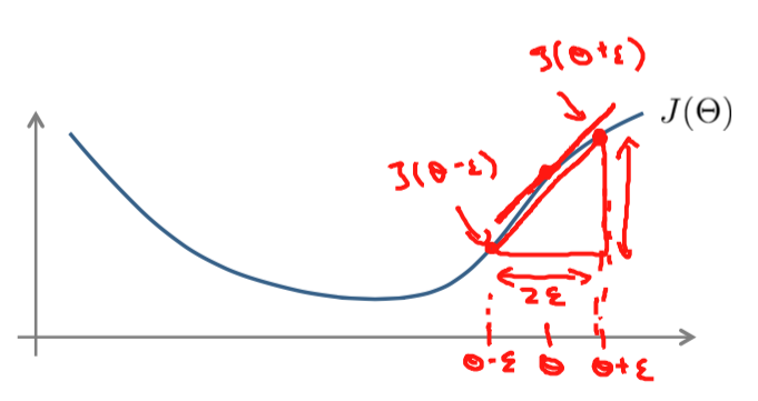
with $\epsilon = 10^{-4}$. The implementation would look like this:
gradApprox = (J(theta + EPSILON) - (J(theta - EPSION)) / (2 * EPSILON)The parameter vector $\theta \mathbb{R}^n$ is the unrolled version of all the $\Theta^{(l)}$. The partial derivitives of the cost function would look like this:
$$\frac{\delta}{\delta \theta_1} J(\theta) = \frac{J(\theta_1 + \epsilon, \theta_2, ..., \theta_n) - J(\theta_1 - \epsilon, \theta_2, ..., \theta_n)}{2 \epsilon}\\ \frac{\delta}{\delta \theta_2} J(\theta) = \frac{J(\theta_1, \theta_2 + \epsilon, ..., \theta_n) - J(\theta_1, \theta_2 - \epsilon, ..., \theta_n)}{2 \epsilon}\\ ... \\ \frac{\delta}{\delta \theta_n} J(\theta) = \frac{J(\theta_1, \theta_2, ..., \theta_n) + \epsilon - J(\theta_1, \theta_2, ..., \theta_n - \epsilon)}{2 \epsilon}\\ $$for i = 1:n,
thetaPlus = theta;
thetaPlus(i) = thetaPlus(i) + EPSILON;
thetaMinus = theta;
thetaPlus(i) = thetaPlus(i) - EPSILON;
gradApprox(i) = (J(thetaPlus) - J(thetaMinus)) / (2*EPSILON);
We then need to check that gradApprox $\approx$ DVec returned from the back propagation.
Implementation Note
- Implement the back propagation to compute
DVec(unrolled $D^{(1)}, D^{(2)}, D^{(3)}$) - Implement numerical gradient checking to compute
gradApprox - Make sure they have similar values
- Turn off gradient checking. Using backprop code for learning.
Important: Be sure to disable gradient checking before training your classifier. If you run numerical gradient computation on every iteration of gradient descent your code will be very slow.
Random Initialization
For gradient descent and advanced optimization method, we need an initial value for $\Theta$.
optTheta = fminunc(@costFunction, initialTheta, options)Consider gradient descent with initialTheta = zeros(n,1).
Zero Initialization
When initialized with zero, after every update the parameters corresponding to the inputs going into each of the hidden units are identical.
Random Initialization: Symmetry Breaking
Initialize each $\Theta^{(l)}_{ij}$ to random value in $[-\epsilon, \epsilon]$. For example:
Theta1 = rand(10,11)*(2*INIT_EPSILON) - INIT_EPSILON;
Theta2 = rand(1, 11)*(2*INIT_EPSILON) - INIT_EPSILON;
Putting it together
- Pick a network architecture (connectivity pattern between neurons)
- Number of inputs: dimensions of features $x^{(i)}$
- Number of output units: number of classes
(Reasonable default: one hidden layer, or if more than one hidden layer, you need to have the same number of hidden units in every hidden layer (usually the more the better))
Training a Neural Network
- Randomly initialize weights
- Implement forward propagation to get $h_\Theta(x^{(i)})$ for any $x^{(i)}$
- Implement code to compute cost function $J(\Theta)$
- Implement back propagation to compute partial derivitives $\frac{\delta}{\delta \Theta^{(l)}_{jk}} J(\Theta)$
For all features:
- Perform forward and backward propagation using the example $(x^{(i)}, y^{(i)})$
- (Get activations $a^{(l)}$ and delta terms $\delta^{(l)}$ for $l=2,…,L$)
- Compute partial derivitive of the cost function
- Use gradient checking to compare $\frac{\delta}{\delta \Theta^{(l)}_{ij}} J(\Theta)$ computed using backpropagation vs. using numerical estimate of gradient of $J(\Theta)$. Turn off code for gradient checking.
- Use gradient descent or adavanced optimization method with backpropagation to try to minimize $J(\Theta)$ as a function of parameters $\Theta$
Week 5
Deciding What to Try Next
Debugging a learning algorithm
Suppose you implemented regularized linear regression. However, when you test your hypothesis on a new set of data, you find that it mameks unacceptably large errors in its predictions. What should you try next?
- Get more training examples
- Try a smaller set of features
- Try getting additional features
- Try adding polynomial features
- Try decreasing $\lambda$
- Try increasing $\lambda$
Machine Learning Diagnostics
Diagnostic: A test that you can run to gain insight what is/isn't working with a learning algorithm, and gain guidance as to how best to improve its performance.
Diagnostics can take itme to implement, but doing so can be very good use of your time.
Evaluating a Hypothesis
To test the hypothesis, the training data gets split into a training set (bigger part) and a test set (smaller part). You could for example split them into 70%/30%. Note that the data is sorted, the picks should be randomized, or the data should be randomly shuffled.
- Training set: $$\begin{array}{c} (x^{(1)},y^{(1)})\\ (x^{(2)},y^{(2)})\\ \vdots \\ (x^{(m)},y^{(m)}) \end{array}$$
- Test set (with $m_\text{test}$: number of examples): $$\begin{array}{c} (x^{(1)}_\text{test},y^{(1)}_\text{test})\\ (x^{(2)}_\text{test},y^{(2)}_\text{test})\\ \vdots \\ (x^{(m)}_\text{test},y^{(m)}_\text{test}) \end{array}$$
Training/Testing Procedure for Linear Regression
Learn parameter $\theta$ from training data (minimizing training error $J(\theta)$ and compute the test set error:
$$ J_\text{test}(\theta) =\frac{1}{2m_\text{test}} \sum^{m_\text{test}}_{i=1} \left( h_\theta(x^{(i)}_\text{test} - y^{(i)}_\text{test}) \right) $$The misclassification error:
$$\text{err}(h_\theta(x), y) = \left\{\begin{array}{l} \text{if} \; h_\theta(x) \geq 0.5 \;\; y=0 \\ \text{or if} \; h_\theta(x) \lt 0.5 \;\; y=1 \end{array}\right.$$The test error is:
$$\frac{1}{m_\text{test}} \sum^{m_\text{test}}_{i=1} \text{err}(h_\theta(x^{(i)}_\text{test}), y^{(i)}_\text{test})$$Model Selection and Train/Validation/Test Sets
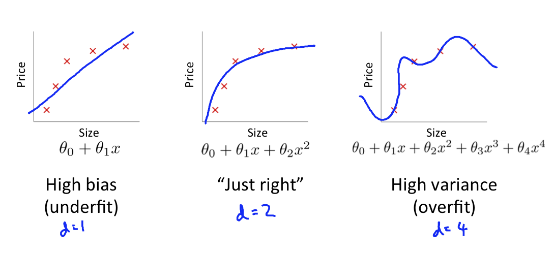
Once parameters $\theta_0, \theta_1, \cdots, \theta_4$ were fit to some data (training set), the error of the parameters as measured on that data (the training error $J(\vec\theta)$) is likely to be lower than the actual generalization error.
Model Selection
- $h_\theta(x) = \theta_0 + \theta_1 x$ with $d=1$ $\rightarrow$ $\Theta^{(1)} \rightarrow J_\text{test}(\Theta^{(1)})$
- $h_\theta(x) = \theta_0 + \theta_1 x + \theta_2 x^2$ with $d=2$ $\rightarrow$ $\Theta^{(2)} \rightarrow J_\text{test}(\Theta^{(2)})$
- $h_\theta(x) = \theta_0 + \theta_1 x + \theta_2 x^2 + \theta_3 x^3$ with $d=3$ $\rightarrow$ $\Theta^{(3)} \rightarrow J_\text{test}(\Theta^{(3)})$
- …
- $h_\theta(x) = \theta_0 + \theta_1 x + \cdots + \theta_10 x^10$ with $d=10$ $\rightarrow$ $\Theta^{(10)} \rightarrow J_\text{test}(\Theta^{(10)})$
In order to select a model you could take the hypothesis with the lowest test set error. (Let's say for now it's $\theta_0 + \cdots + \theta_5x^5$). Now how well does it generalize? report the test set error $J_\text{test}(\theta^{(5)}$
The problem is, that $J_\text{test}(\theta^{(5)}$ is likely to be an optimistic estimate of generalization error, i.e. our extra parameter ($d$ = degree of polynomial) is fit to the test set.
Now instead of splitting it 70/30 we split the dataset like this: 60% training set, 20% cross validation set ($cv$) and 20% test set.
- $$\begin{array}{c} (x^{(1)}, y^{(1)})\\ (x^{(2)}, y^{(2)})\\ \vdots\\ (x^{(m)}, y^{(m)})\\ \end{array}$$
- $$\begin{array}{c} (x^{(1)}_{cv}, y^{(1)}_{cv})\\ (x^{(2)}_{cv}, y^{(2)}_{cv})\\ \vdots\\ (x^{(m)}_{cv}, y^{(m)}_{cv})\\ \end{array}$$
- $$\begin{array}{c} (x^{(1)}_{\text{test}}, y^{(1)}_{\text{test}})\\ (x^{(2)}_{\text{test}}, y^{(2)}_{\text{test}})\\ \vdots\\ (x^{(m)}_{\text{test}}, y^{(m)}_{\text{test}})\\ \end{array}$$
Where $m_{cv}$ is the number of cross validation examples.
- Training error: $J(\theta) = \frac{1}{2m} \sum^{m}_{i=1} (h_\theta(x^{(i)})-y^{(i)})^2$
- Cross Validation error: $J_{cv}(\theta) = \frac{1}{2m_{cv}} \sum^{m_cv}_{i=1} (h_\theta(x^{(i)}_{cv})-y^{(i)}_{cv})^2$
- Cross Validation error: $J_{\text{test}}(\theta) = \frac{1}{2m_\text{test}} \sum^{m_\text{test}}_{i=1} (h_\theta(x^{(i)}_{\text{test}})-y^{(i)}_{\text{test}})^2$
Now to select a model you calculate $min_\theta J(\theta)$ for $\theta^{(i)}$ and then calculate $J_{cv}(\theta)$. You then select the model with the lowest cross validation error.
Diagnosing Bias vs. Variance
Suppose your learning algorithm is performing less wellt han yoh were hoping. ($J_{cv}(\theta)$ or $J_\text{test}(\theta)$ is high.) Is it as bias problem or a variance problem?
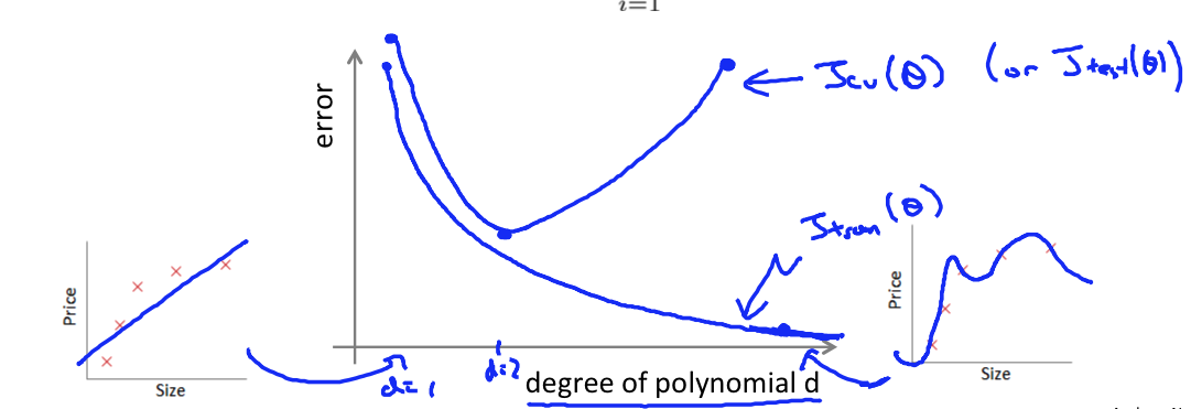
- Bias (underfit): $J_\text{train}(\theta)$ will be high, $J_{cv}(\theta) \approx J_\text{train}(\theta)$
- Variance (overfit): $J_\text{train}(\theta)$ will be low, $J_{cv}(\theta) \gt\gt J_\text{train}(\theta)$
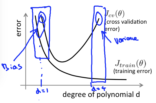
Regularization and Bias/Variance
Linear Regression with Regularization
Choosing the Regularization Parameter $\lambda$
Bias/Variance as a Function of the Regularization Parameter $\lambda$
Learning Curves
Appendix
Footnotes
- Taken from the Machine Learning Video Lecture: »What is Machine Learning?«, Minute
01:49at Coursera